Event-Based Analytics Pitfalls

Event-based analytics is a way to analyze information systems that relies on the law of large numbers. The stream of discrete events generated by the system is written into a data store together with metadata that captures the context of each event: time, geo, session/user IDs, traffic source, and so on. The resulting corpus of events is then used to segment users into cohorts, build funnels, and calculate metrics, i.e., causal relationships between events are inferred statistically. Event-based analytics has become the de facto standard (Mixpanel, Amplitude, Google Analytics, etc.), replacing the older session-based approach. However, this approach comes with several fundamental issues.

Time is a way to order active causes and accumulating effects.

Alexey Semikhatov. Walks Through the Restless Universe.

Every event in a typical analytics system contains a single required field—the event name (for instance, event_name) that uniquely identifies the event type. Stability ends there: every other parameter is optional or unreliable. Consider the example below:

{
  "event_name": "order_paid",
  "timestamp": "2026-02-07T10:12:33.120Z",
  "user_id": "u_123",
  "session_id": "s_456",
  "properties": { "amount": 1290, "currency": "RUB", "method": "apple_pay" },
  "context": { "app_version": "7.1.0", "os": "iOS", "locale": "ru_RU" }
}

The timestamp field captures when the event was recorded. Modern information systems are overwhelmingly distributed, which inevitably means clock drift between the server and clients. If we define timestamp as the moment the event reaches a single central server, this value includes the time spent traveling across the network. Events may be created in one order but arrive in another. If we define timestamp as the moment the client creates the event, the server can no longer guarantee the correct temporal ordering of different clients’ events. In practice, it is impossible to establish a causal order of events reliably using timestamp alone.

In theory, the user_id and session_id fields allow us to identify which group an event belongs to. But what if the user’s cookies were wiped for whatever reason? You can drop such events altogether, yet that means immediate data loss and poorer representativeness of the overall dataset.

The context field is generally derived from the system’s technical parameters and has historically been used to identify the client (user agent, unique device ID, etc.). Over time, client platforms (browsers and mobile OSs) have tightened the screws by blocking user-tracking mechanisms. Today, you can no longer rely on context unequivocally.

The properties field describes application-level context. Technically you can pack a lot of information into it, but in high-throughput systems every byte in an event payload turns into gigabytes of extra traffic. You cannot squeeze “everything” into properties, so you end up rebuilding event relationships through shared context on a case-by-case basis.

As a result, events are recorded fragmentarily—isolated from one another. Analysts still need to derive causal relationships between events to reach any conclusions. This is like putting War and Peace through a shredder: the output certainly contains data, but how do you extract meaning? Hence the first limitation of event-based analytics in an unsynchronized world: you need A/B tests to uncover causality.

A second fundamental issue is that event sequences suffer from missing and duplicate requests. In theory, to log a client-side event (for example, tapping “Order”), the client should issue an idempotent request to the analytics system—guaranteeing that the event is recorded exactly once. In practice, the event stream is extremely intense, so events are usually recorded without uniqueness checks to keep ingestion fast. Such checks require comparing identifiers—that is, additional reads. Caches can help, yet they always limit the size of the deduplication window. Moreover, as noted above, events are generally not linked to one another. If two events do not share a user_id, it’s hard to distinguish a retry caused by a network glitch from a repeated user action. Missing requests are equally hard to detect. Consequently, duplicates and gaps in the raw data make running statistically significant A/B tests much harder.

Together, these two fundamental limitations create several applied problems that surface regardless of how advanced your tooling is.

First, organizations tend to embrace quantitative analytics seriously only once intuition starts to fail. Intuition works great on “low-hanging fruit”—obvious ideas and common sense shaped by a specific person’s experience. Once the low-hanging fruit is gone, you have to accept a smaller minimal detectable difference, and at small magnitudes you suddenly need “real” math. The A/B-test calculator shows that shrinking the Minimum Detectable Effect tenfold increases the Sample size one hundredfold, and a hundredfold reduction in the minimal effect inflates the sample ten thousand times! In other words, the cost of experimentation grows quadratically.

// 5%
Baseline conversion rate: 20%
Minimum Detectable Effect: 5%
Statistical power 1−β: 80%
Significance level α: 5%
Question: How many subjects are needed for an A/B test?
Answer: 1030 per variation

// 0.5%
Baseline conversion rate: 20%
Minimum Detectable Effect: 0.5%
Statistical power 1−β: 80%
Significance level α: 5%
Question: How many subjects are needed for an A/B test?
Answer: 100746 per variation

// 0.05%
Baseline conversion rate: 20%
Minimum Detectable Effect: 0.05%
Statistical power 1−β: 80%
Significance level α: 5%
Question: How many subjects are needed for an A/B test?
Answer: 10049393 per variation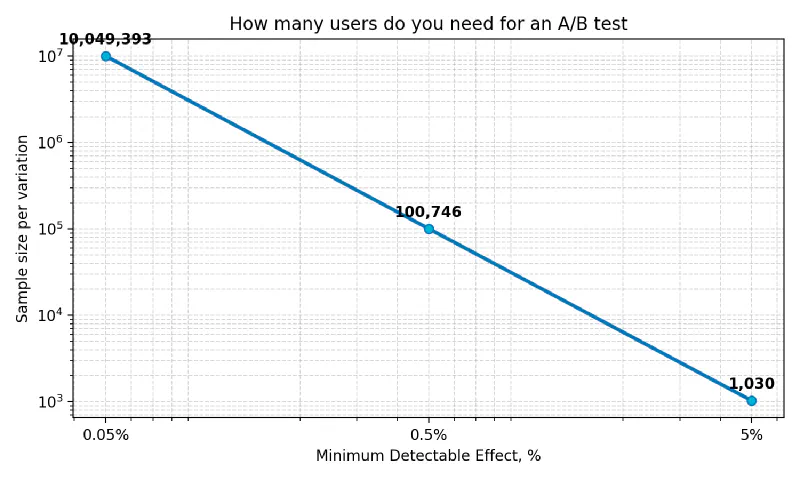

Larger samples translate into higher costs: you either need a bigger audience or you must run the test longer, depriving other experiments of traffic. Long means expensive!

Moreover, a drawn-out experiment can undermine how fast you make decisions. A statistical effect visible during the experiment may become irrelevant by the time you ship the change, especially if too much time has passed. For example, vacation rentals in resort regions have highly seasonal demand.

Second, averaging across a large sample can wipe out local effects. One part of the audience may respond positively to the experiment, while another reacts negatively. The aggregate A/B test “doesn’t light up,” even though each cohort shows a strong effect on its own. By averaging, we risk building a service that is equally inconvenient for everyone. To split the audience into behaviorally homogeneous cohorts, analysts perform lots of manual work to identify suitable covariates and then cohort by them. The hope is that getting statistical significance in an individual cohort will be easier. In general, however, searching for covariates again leans on “common sense”: you keep launching experiments without any guarantee of results.

Third, landing a user in a particular cohort does not guarantee homogeneous behavior. Once you shrink the sample by running an experiment inside a cohort, the role of individual confounders skyrockets. The same user can make one decision in the morning when fresh and another in the evening when exhausted. Results from a morning experiment no longer apply to that user’s “evening” state. Cutting the sample reduces the robustness of the chosen covariate combination and often makes it unusable for personalization tasks.

Thus, analytics built on A/B tests yields mathematically guaranteed results, but the mathematical “price” of significance is inflexible and may be unacceptable. Attempts to lower that price via preprocessing lead to higher analyst/developer labor costs and drastically more complex event-analytics pipelines. Hunting for alternative metrics that are more sensitive to a “gray” A/B test bloats the metric suite, making subsequent business analysis harder.

Event tracing can act as an “accelerator” of event-based analytics by making causes and effects explicit as parent-child relationships between events. A parent event may be a cause (or precondition) for its child event, yet the child cannot cause the parent. To achieve this, your system architecture must guarantee that every event has its own unique uuid (for example, UUID v4) and a parent_uuid that points to its ancestor. For root events, parent_uuid can be null or omitted entirely:

{
  "uuid": "b9172231-b37f-436e-b8fc-e73e762f2dac",
  "parent_uuid": "c40435de-e822-4ea5-adb0-8d63ca083d16",
  "event_name": "order_paid",
  "timestamp": "2026-02-07T10:12:33.120Z",
  "user_id": "u_123",
  "session_id": "s_456",
  "properties": { "amount": 1290, "currency": "RUB", "method": "apple_pay" },
  "context": { "app_version": "7.1.0", "os": "iOS", "locale": "ru_RU" }
}

This guarantee lets us detect the processes unfolding inside information systems per user, directly. We can still employ the law of large numbers and A/B tests, but now the “feedstock” is fundamentally different.

Behavior is a dependence of some value on time.

Alexey Semikhatov. Walks Through the Restless Universe.

First, analyzing and comparing individual traces allows us to replace the manual hunt for covariates and confounders with automatic cohorting by chain structure—in other words, cohorting by behavior. If a group of users exhibits similar behavior under the same conditions, their unique mix of confounders is likely to produce a similar reaction to the experiment. It’s easier to reach statistical significance in such a cohort.

Second, with per-user behavior traces in hand we can tell whether a user also participated in another experiment. This makes it safer to split traffic among multiple simultaneous experiments and increase the “clean” sample size for each one.

Finally, analyzing traces after the experiment lets us observe how AB-test sensitivity changes step-by-step at every span in the chain. We can automatically determine the metric or set of metrics that the experiment influences.

Event-based analytics has several fundamental and applied problems. Still, we can largely mitigate them by embracing event tracing.

Yury Dubovoy (Docingem), February 9, 2026.